Figure 47 of the ADS8860 data sheet also provides an input sampling stage equivalent circuit, which provides a starting point for construction of a sampling stage circuit for simulation. Here, a series of voltage controlled switches can be implemented to effectively create a model of this topology in simulation:

Figure 4-4 ADS8860 Switching Simulation Model

In this model, the voltage sources at the bottom effectively create pulse widths, where the left source generates the acquisition time of the device, and the right generates the conversion time. It should be noted that for this simulation, the conversion time is handled simply as a small pulse at the end of the sampling period to create a worst case voltage droop and secure a more robust testing scenario.

Next, the INA293 SPICE model, the charge bucket filter, and the ADS8860 switching model are connected together, resulting in a final simulation environment that can be used to validate stability and settling accuracy. If the device is capable of converging under this use case, it can be inferred that the device should be capable of responding to any other value inside the sample and hold time. However, prior to beginning analysis, the steady state value of the error must be calibrated. This allows the model to ignore other error contributions here, such as offset of the amplifier, and examine only the switching models ability to settle to steady state. This is achieved by performing a DC steady state analysis simulation with the model under full-scale input, steady-state output constraints. Once the steady state output is known, the value of the error reference is updated to this value so that, should the simulation perform as expected, the error shown in the simulation will converge to zero. The necessary portions to be observed and changed are indicated in Steady State Error Calibration Information:

Figure 4-5 Steady State Error Calibration Information

With the system calibrated to steady state, data can now be captured. For the simulation data captured in Initial Simulation Results below, the filter is examined at the calculated C_FILT, 1200pF, and its corresponding R_{FILT, MAX} of 59.1Ω (note that for the single ended #2 topology, this resistance is split between the resistors on each leg of the ADC). The maximum resistance was chosen here, as by earlier calculations, it was shown that resistance should be greater than 89Ω for stability purposes. The goal is to examine the response of the device under given parameters of the Analog Engineer's Calculator before making adjustments to the design. The amended schematic and its corresponding output is shown in the figures below.

Figure 4-6 Full Initial Simulation Schematic

Figure 4-7 Sample and Hold Initial Waveforms

It can be seen by inspection in the initial simulation that the output is still in the process of settling in this configuration. The data shows that the output is not fully settled, and this demonstrates as observed earlier that the device cannot drive the ADS8860 in this configuration without some amount of data loss. There are several avenues to be investigated at this point: the filter values can be re-evaluated, the output of the INA293 can be buffered with a device that possesses the bandwidth to properly drive the device at this sampling rate, or, with certain devices such as the ADS8860, the sampling clock can be relaxed to extend the acquisition time to an acceptable level.

An issue also presents itself here from earlier analysis, in that a resistor value larger than 89Ω is needed to guarantee stability (for 1200pF). This means that with the calculated values of R_FILT by the assumptions made, for all cases shown, we risk instability in the system. This needs to be balanced, however. While a higher value of R_FILT helps mitigate amplifier stability issues, this resistance also adds distortion as a result of interactions with the nonlinear input impedance of the ADC. This distortion increases with the added resistance, input signal frequency, and input signal amplitude. Therefore, the selection of R_FILT requires balancing the stability of the driver amplifier and distortion performance of the design.

As the bandwidth needs of the system in this current configuration are greater than can be provided by the INA293, a final option exists before designing in a buffer: relaxation of the sampling clock of the ADC. While 1MSPS with this device looks unachievable, in many modern ADCs, t_sample is calculated as the sum of t_acq and t_conv, where t_conv is a fixed parameter inside the ADC that is generated by an internal clock, but the acquisition time is determined from an external clock provided to the ADC to establish the sampling rate. This means that if the device is sampled at a rate below its default sample rate, the time added to the sampling period effectively increases the time of t_acq, allowing the INA293 additional time to settle. From the mathematics discussed in The ADC Charge Bucket Filter, it can also be shown that relaxation of the sampling period also provides a larger selection of R_FILT. Furthermore, a combination of these equations can be rearranged to demonstrate that for a given bandwidth, resolution, and filter network, the acquisition time needed for proper settling is

Equation 22.

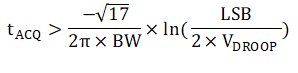
For the INA293, the closed loop bandwidth of the A1 variant is 1.3MHz. Using the above equation, it can be derived that with this bandwidth, the INA293 needs approximately 4.1µs to properly drive an ADC with a filter designed inside the calculated criterion. Note that the derivations for C_FILT are primarily based off of the sample and hold capacitance C_SH, and therefore do not change from the initial design. The range of R_FILT however, is increased as a result of this change in sample rate, and now provides selectable values inside a range that are above the stability criterion derived earlier. For ease of clock generation, a new sampling period of 5µs is chosen, and as conversion time remains the same at 710ns, the new acquisition time is now 4.29µs.

A 200kHz sampling rate is simulated in ADS8860 Adjusted Response, f_sample = 200kHz. The minimum calculated RFILT of 104.4Ω is split across the charge bucket filter. The second image is a closer look at the error signal inside of a single acquisition period.

Figure 4-8 ADS8860 Adjusted Response, f_sample = 200kHz

Figure 4-9 ADS8860 Error Response, fsample = 200kHz, R_FILT = 104.4Ω

It can now be observed that the amplifier has room to settle and converges to well inside 1/2 LSB inside the acquisition time. However, this does not complete the design. The final technique to discuss is optimization of the error response. While a range of resistances based on approximation is a good starting point, there is merit in examining the effect of this resistance over a range of values to optimize the response of the amplifiers settling. Inside the simulation, it is possible to test a range of values for R_FILT, and observe how the response is shaped in relation to these resistance values. A range of 50Ω to 150Ω is shown in Effects of R_FILT on Error Response.

Figure 4-10 Effects of R_FILT on Error Response

Examining the effects of these resistances on the output impedance of the amplifier and the 1200pF capacitor, it can be observed that the impedance curve softens as additional resistance is added, beginning to converge towards a well dampened response around 130Ω:

Figure 4-11 AC Response of INA293 With Various R_FILT

If necessary, additional iterations can be made inside of these values to further tighten resistances. However, 130Ω is chosen here, as it provides a reasonably damped response while still providing proper settling inside the acquisition window to -10.29uV. Finally, note that the final settled value is slightly higher than the previous iteration. This is due to distortion added from the increased value of resistance, but still allows the design to settle within the required range.