SBOA550 October 2022 OPA1671 , OPA2990 , SN74HCS04 , SN74HCS164 , SN74HCS30 , SN74LVC1G00 , SN74LVC1G123 , TLC04 , TLC14 , TS5A9411
- Abstract
- Trademarks
- 1 Introduction
- 2 The Davies Generator
- 3 Optimizing Standard Resistance Values for THD Performance
- 4 Simulation Examples
- 5 Compensating for Shift Register Output Resistance
- 6 Voltage-Mode Thevenin Equivalent
- 7 Harmonic Filtering
- 8 Tracking Harmonic Filter
- 9 Multiphase Output
- 10Conclusion
- 11Acknowledgment
- 12References
- A Analytical Solution for Resistance Network Values
- B Forbidden States of the Johnson Counter
4 Simulation Examples
Using the values from Section 3 and assuming no random resistor variation, the following TINA-TI SPICE simulation of Figure 4-1 based on the SN74HCS164 shift register demonstrates the upper limit of THD performance while using a realistic model of the shift register but neglecting the output resistance. Using 0-V, +5-V logic levels as shown results in a common-mode DC offset of 2.5 V in the output. Depending on the application, subsequent circuit stages can require AC coupling or some other method to remove the offset if it is undesirable. The additional 1-kHz square-wave source shown is used as a reference to sanity-check the simulated THD estimates since the Fourier series is well known. The scaled mid-supply common-mode voltage, VCM, provides the virtual ground that the op amp of Figure 2-1 otherwise provides.
Clocking the circuit at 16 kHz results in an 8 × oversampled 1-kHz stepped-sinusoidal current into the virtual ground node, along with the reference square wave current.
From within the TINA-TI diagram window, each curve is selected and a Fourier analysis estimates THD. As a sampled data system, only harmonics in the first Nyquist zone are considered and higher Nyquist zones ignored. This indicates that even without harmonic filtering < 0.17% THD is achieved, see Figure 4-3 and Figure 4-4.
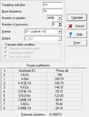 Figure 4-3 Simulated THD Results of
Stepped Sinusoid Compared to Reference Square Wave
Figure 4-3 Simulated THD Results of
Stepped Sinusoid Compared to Reference Square Wave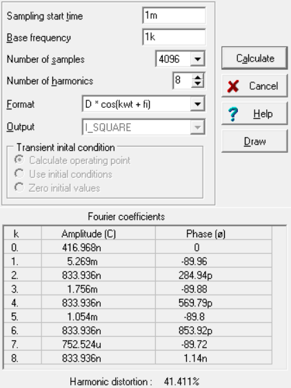 Figure 4-4 Simulated THD Results of
Stepped Sinusoid Which Shows > 47-dB Improvement in 3rd
Harmonic Suppression
Figure 4-4 Simulated THD Results of
Stepped Sinusoid Which Shows > 47-dB Improvement in 3rd
Harmonic SuppressionThe Fourier expansion of an ideal square wave is where . From this expansion it is clear the ratio of the 3rd harmonic to the fundamental is 1/3 (–9.54 dB) and verified in simulation in Figure 4-4. This indicates the TINA-TI THD computation appears correct. The 3rd harmonic of the stepped sinusoid is –57.2 dB relative to the fundamental, a > 47-dB improvement over the square wave.